これまでは正解ラベルがある前提、つまり教師あり学習でモデルを構築した。今回は正解ラベルがない前提でモデルを構築する。
教師なし学習としては混合ガウスモデルを利用する。
内容
- データの読み込み、前処理
- モデルの構築
- プロット
データの読み込み、前処理
データの読み込み、前処理はこれまでと同様である。
import matplotlib.pyplot as plt
%matplotlib inline
import seaborn as sns
import numpy as np

# データセット読み込み
iris = sns.load_dataset('iris')
iris.head()

# データ前処理
X_iris = iris.drop('species', axis=1)
X_iris.head()
モデルの構築
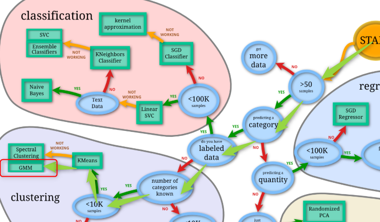
混合ガウスモデルはsklearn.mixture.GaussianMixureを利用する。
from sklearn.mixture import GaussianMixture as gm
model = gm(n_components=3,covariance_type='full')
model.fit(X_iris)
y_gmm = model.predict(X_iris)
print(y_gmm)
# [0 0 0 0 0 0 0 0 0 0 0 0 0 0 0 0 0 0 0 0 0 0 0 0 0 0 0 0 0 0 0 0 0 0 0 0 0
 0 0 0 0 0 0 0 0 0 0 0 0 0 2 2 2 2 2 2 2 2 2 2 2 2 2 2 2 2 2 2 1 2 1 2 1 2
 2 2 2 1 2 2 2 2 2 1 2 2 2 2 2 2 2 2 2 2 2 2 2 2 2 2 1 1 1 1 1 1 1 1 1 1 1
 1 1 1 1 1 1 1 1 1 1 1 1 1 1 1 1 1 1 1 1 1 1 1 1 1 1 1 1 1 1 1 1 1 1 1 1 1
 1 1]
プロット
2次元にプロットするためにはPCAで2次元にする。
from sklearn.decomposition import PCA
pca = PCA(n_components=2)
pca.fit(X_iris)
pca_transformed = pca.transform(X_iris)
# データマージ
iris["PCA1"] = pca_transformed[:, 0]
iris["PCA2"] = pca_transformed[:, 1]
さらにy_gmmもマージする。
iris["cluster"] = y_gmm

iris.head()
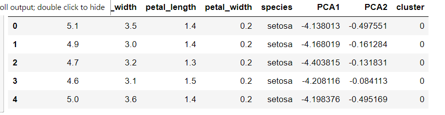
PCA1, 2およびクラスタがすべての一つのデータフレームに収まったのでプロットして検証する。
sns.lmplot("PCA1", "PCA2", hue='species', data=iris, fit_reg=False);
sns.lmplot("PCA1", "PCA2", hue='cluster', data=iris, fit_reg=False);
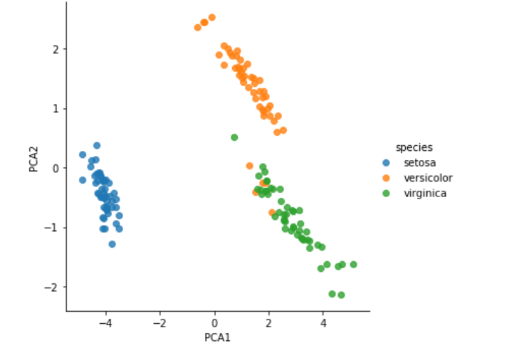
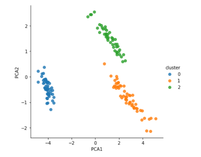
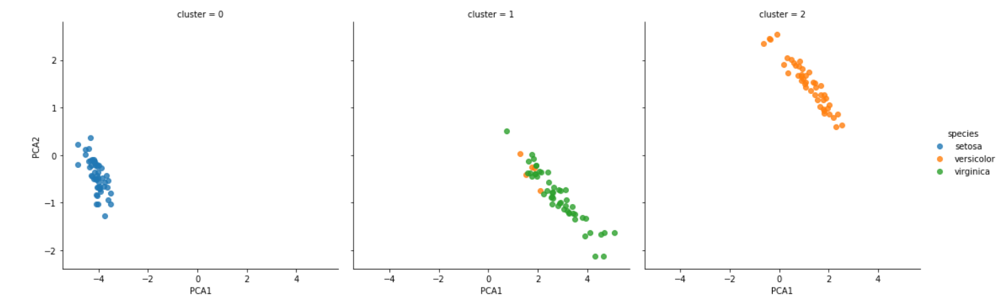
gmmはほぼ正しく分類できている。seaborn.lmplotはhueのほかにcolを利用してさらにグラフを分割することができる。
hue, col, row : strings
Variables that define subsets of the data, which will be drawn on separate facets in the grid. See the*_orderparameters to control the order of levels of this variable.
sns.lmplot("PCA1", "PCA2", hue='species', col="cluster", data=iris, fit_reg=False);